Remote Sensing | Machine Learning | PYTHON HANDSON

Auto Encoders for Land Cover Classification in Hyperspectral Images

Part 2: Auto Encoders for land cover classification in Hyperspectral Images using K-Nearest Neighbor Classifier(K-NNC), Support Vector Machine(SVM), and Gradient Boosting using Python.

Photo by NASA on Unsplash

Table of Contents

1. Quick Recap
2. K-Nearest Neighbor Classifier
3. Support Vector Machine
4. Gradient Boosting
5. Conclusion
6. References

Quick Recap

A hyperspectral image is an image cube with the shape of R x C x B. where R and C are the image's height and width. B represents the no. of bands in the image.

Dimensionality reduction has been one of the important aspects of building efficient machine learning models. It is a statistical technique used to reduce vast dimensions of the data to lesser dimensions with minimal loss of information.

Feature Selection: selecting important features/bands of the data which has more importance. Different ranking methods are used to select bands of the hyperspectral image. Here are the useful research papers to dive into band selection/ranking.

Methodology for Hyperspectral Band Selection

A Novel Ranking-Based Clustering Approach for Hyperspectral Band Selection

Salient Band Selection for Hyperspectral Image Classification via Manifold Ranking

Feature Extraction: It is a process of converting higher dimensional data to lesser dimensions using statistical methods like Singular Value Decomposition (SVD), Principal Component Analysis (PCA), Linear Discriminant Analysis (LDA), t-Stochastic Neighborhood Embedding (t-SNE), e.t.c. Here are useful research papers to know more about Feature extraction in Hyperspectral Images.

Comparative study of feature extraction techniques for hyperspectral remote sensing image…

Semisupervised Local Discriminant Analysis for Feature Extraction in Hyperspectral Images

The previous article, “AutoEncoders for Land Cover Classification of Hyperspectral Images — Part -1” covers the Auto Encoder implementation, which is further used to reduce the dimensions(103 to 60) of the Pavia University Hyperspectral Image.

AutoEncoders for Land Cover Classification of Hyperspectral Images — Part -1

Let’s revisit the Pavia University Hyperspectral image data. The Pavia University is captured by ROSIS sensor over Pavia, Northern Italy. It has 103 spectral bands with dimensions of 610 x 340. The data is publically available and I have created this Kaggle dataset for better reach and accessibility.

Pavia University HSI

Let’s visualize the data before diving into the Auto Encoders for land classification of Pavia University. Let’s read the data:

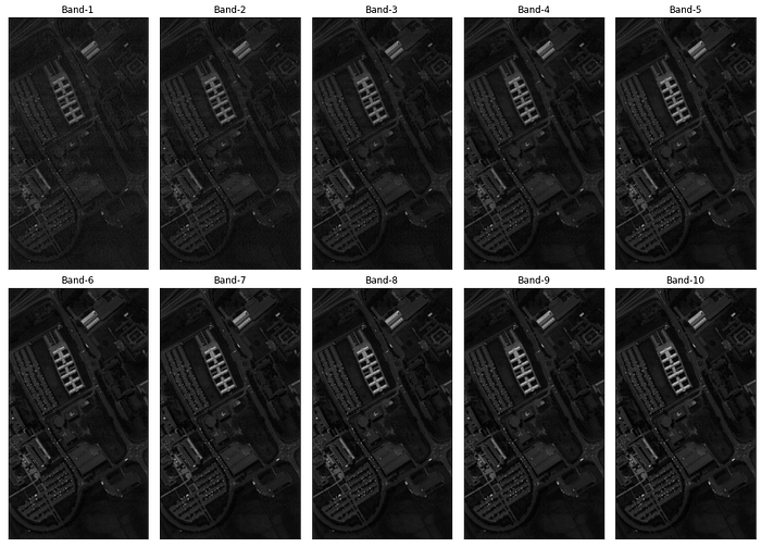
The code reads the data from the Kaggle dataset and shows the dimensions of the data. Let’s visualize the bands of the data. The below code shows the first 10 bands of the Pavia university HSI using the earthpy package.

Visualization of Bands of the Pavia University — Image by Author

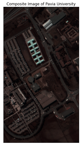
The HSI image has multiple bands, it is hard to see the details using a single band. Thus an RGB composite image helps us to better understand the hyperspectral image. The below code shows the RGB composite image using the bands (36, 17, 11).

Image by Author

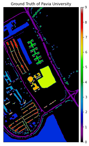
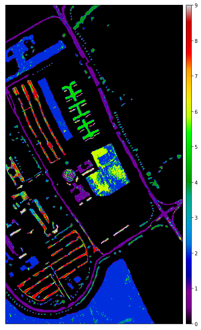
The ground truth of Pavia University Image has 9 classes and the labels with no class are represented in black color.

Image by Author

Auto-Encoder

AutoEncoder is an unsupervised dimensionality reduction technique in which we make use of neural networks for the task of Representation Learning. Representation learning is learning representations of input data by transforming it, which makes it easier to perform a task like classification or Clustering. A typical autoencoder consists of three components. They are:

Encoder: The encoder consists of a set of neural network layers with gradually decreasing nodes in each layer. The goal is to represent higher dimensional data to lower-dimensional data. The encoder can be represented as an equation. where ‘E’ is the encoder, ‘X’ is the higher dimensional data, and ‘x’ is the latent representation of the data.

Encoder — Image by Author

Latent View Representation: It is the lowest possible presentation of the data. using the latent view representation the decoder will try to reconstruct the original data.

Decoder: The decoder is a set of neural network layers with gradually increasing nodes in each layer. The goal is to represent the original data using the latent view representation. The decoder can be represented as the ‘D’, ‘x’ is the latent view representation and ‘X’ is the higher dimensional data.

Decoder — Image by Author

The reconstruction loss is the measure of the difference between reconstructed and original data. The below equation represents the reconstruction loss.

Reconstruction Loss — Image by Author

The autoencoder needs to be fine-tuned to minimize the reconstruction loss to achieve better results. The Autoencoder architecture used to reduce the dimensions of the Pavia University HSI data is shown below.

The architecture of AutoEncoder — Image by Author

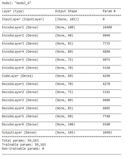
After training the autoencoder the encoder part is taken to reduce the dimensions of the data. Here is the encode architecture:

The architecture of Encoder — Image by Author

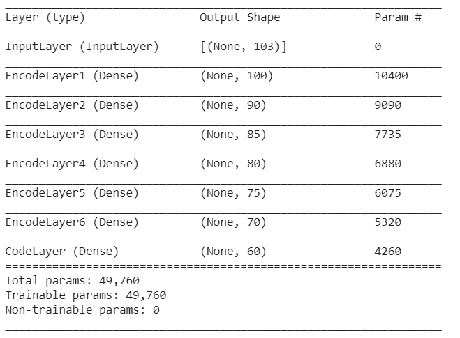
The dimensions of the data were reduced from 103 to 60 and added the class labels to pixels. Here are the first five rows of the data.

Before going on applying classification techniques to the data. Let’s divide the data into train and test in the ratio of 30:70. The pixels with class ‘0’ are ignored during classification as they don’t hold any information. The train and test data have the shape (12832, 60) and (29944, 60).

K-Nearest Neighbor Classifier

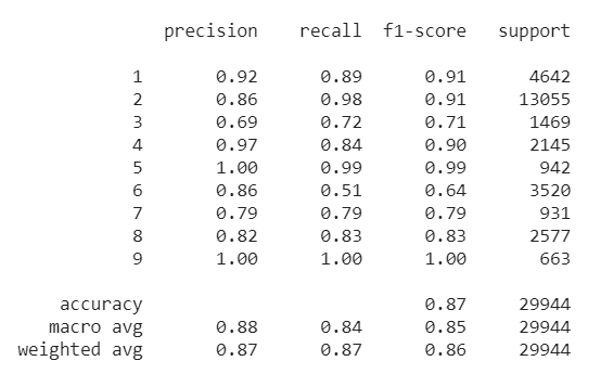
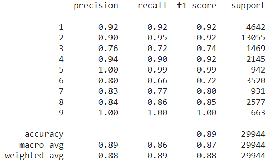
K-Nearest Neighbor is one of the widely used machine learning algorithms for classification tasks. The objective of this method is to find the class of the unknown data instance based on the distance between the test data. The closer the distance between the test instance and the unknown data instance they share a similar class. The below code uses KNeighborsClassifier from Sklearn package to predict the labels of the test data and it also shows the classification report.

Classification Report of KNN on Test Data — Image by Author

The below code is used to predict the labels using the classifier(KNN, SQM, or LGB classifier) and returns the predictions as a numpy array.

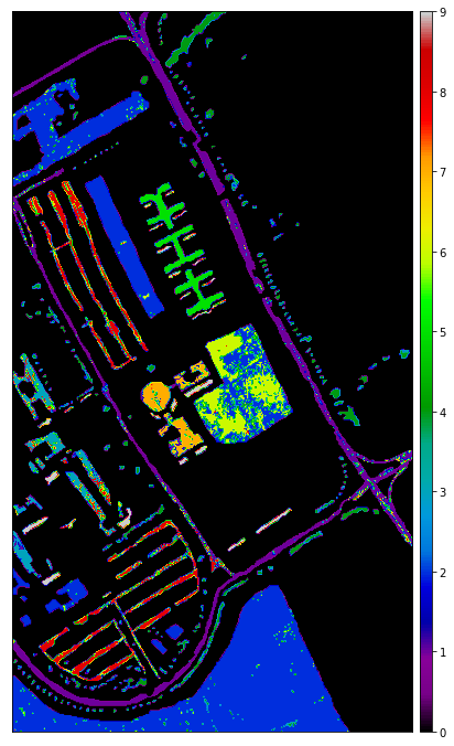
Let’s see the classification map using the KNN classifier. The below code uses the plot_bands() method from the earthpy package.

Classification Map of Pavia University using KNNC — Image by Author

Support Vector Machine

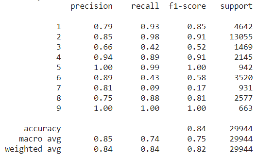
Support Vector Machine is a supervised Machine Learning algorithm that can be used for both classification and regression tasks. It uses a technique called ‘Kernel Trick’ which transforms data to find optimal boundaries to classify the data. The below code is used to implement SVM and predicts the labels of the test data and shows the classification report and classification map.

Classification Report of SVM on Test Data — Image by Author

Classification Map of Pavia University using SVM— Image by Author

Gradient Boosting

Gradient Boosting can be used for classification, regression, and other tasks. It uses a group of weak learners(typically decision trees) and makes it into strong predictors. It generally outperforms the random forest classifier. We are going to use the Light Gradient Boosting(lightgbm) package to implement the gradient boosting classifier. It takes comparatively less time and cost-efficient than other gradient boosting methods.

The below code implements the gradient boosting classifier and shows the classification report and classification map.

Classification Report of SVM on Test Data — Image by Author

Classification Map of Pavia University using LGB— Image by Author

Conclusion

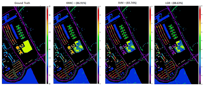
This article covers how to use autoencoders for dimensionality reduction and uses different classifiers such as K-Nearest Neighbor, Support Vector Machine, and Light Gradient Boosting methods on Pavia University Hyperspectral Image. Here is the comparison of classification maps with Accuracy and the ground truth of the Pavia University HSI.

Comparision of Classifier’s with Ground truth of Pavia University — Image by Author

The data and code shown in this article can be accessed using the below links.

Happy Learning. ✨

Starter Notebook - Pavia University HSI Analysis

syamkakarla98/Hyperspectral_Image_Analysis_Simplified

References

Dimensionality Reduction in Hyperspectral Images using Python

Exploratory Data Analysis(EDA) on Satellite Imagery Using EarthPy

Dimensionality Reduction in Hyperspectral Images Using Auto-encoders

Hyperspectral Remote Sensing Scenes

More content at plainenglish.io